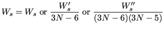
The optimal parameters of the Force Field

The best FF parameters in order to represent the internal molecular motion are obtained by minimizing the following objective function, written as a sum over the considered molecular geometries

$$I=\sum_{g=0}^{N_g} I_g$$ (34)

where

$$I_g = W_g \left[ (E_g-E_0) - V_g \right]^2 + \sum _{K=1}^{3N-6} \frac{W_{Kg}^{\prime}} {3N-6} \left[ E_{Kg}^{\prime} -V_{Kg}^{\prime}\right] ^{2} +$$

$$\sum_{K\leq L}^{3N-6} \frac{2W_{KLg}^{\prime\prime}}{(3N-6) (3N-5) } \left[ E_{KLg}^{\prime\prime}-V_{KLg}^{\prime\prime }\right] ^2$$ (35)

The indexes $K,L$ (capital letters) run over the normal coordinates and include all the modes except for the rotational and translational ones. $E_{g}$ is the total energy obtained by a QM calculation and $E_{0}$ is the same at the reference geometry ($g=0$). $E_{Kg}^{\prime}$ ( $E_{KLg}^{\prime\prime}$) is the energy gradient (Hessian) at a given geometry with respect to the NC evaluated at the same geometry. $V$, $V^{\prime}$ and $V^{\prime\prime}$ are the corresponding quantities calculated by the FF in equation (6). The constants $W$, $W^{\prime}$ and $W^{\prime\prime}$ weight the several terms at each geometry and can be chosen in order to drive the results depending on the circumstances. The energy, gradient and Hessian terms are normalized in order to account for the different number of terms and to make the weights independent from the number of atoms in the molecule.

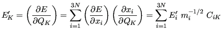
To compute the energy derivatives entering the merit function (35) we have to perform some transformations since no derivative is originally expressed with respect to the NCs. Indeed standard quantum chemistry programs provide derivatives $E^{\prime}$ and $E^{\prime\prime}$ with respect to CCs. Using the above relations and exploiting the completeness of the CCs, the transformation is simple

$$E_K^{\prime} = \left(\frac{\partial E}{\partial Q_K}\right) = \su... ...al x_i}{\partial Q_K}\right) = \sum_{i=1}^{3N}E_i^{\prime }\ m_i^{-1/2}\ C_{iK}$$ (36)

or, in matrix form

$$[E^{\prime}]_{NC} = \widetilde{C} M^{-1/2} [E^{\prime}]_{CC}$$ (37)

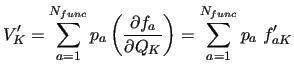
where the square parentheses indicates column vectors of energy gradients computed with respect to the NCs and the CCs. The FF energy gradients at a given geometry

$$V_K^{\prime} = \sum_{a=1}^{N_{func}}p_a \left(\frac{\partial f_a} {\partial Q_{K}}\right) = \sum_{a=1}^{N_{func}}p_a\ f_{aK}^{\prime}$$ (38)

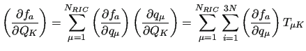
can be conveniently computed using the derivatives of the basis function with respect to the RICs, that is

$$\left( \frac{\partial f_a}{\partial Q_K}\right) = \sum_{\mu=1}^{N... ...IC}} \sum_{i=1}^{3N} \left(\frac{\partial f_a}{\partial q_\mu}\right) T_{\mu K}$$ (39)

or in matrix form

$$[f_a^{\prime}]_{NC} = \widetilde{T} [ f_a^{\prime }]_{RIC}$$ (40)

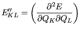
The Hessian matrix of the QM calculation in NCs

$$E_{KL}^{\prime\prime} = \left(\frac{\partial^2E} {\partial Q_K\partial Q_L}\right)$$ (41)

is obtained from the Hessian matrix in the CC basis according to

$$[E^{\prime\prime}]_{NC} = \widetilde{C} M^{-1/2} [E^{\prime\prime}]_{CC} M^{-1/2} C$$ (42)

The second derivatives of the FF are a bit more complicated since they involve derivatives of the $B$ matrix and are conveniently expressed in explicit form

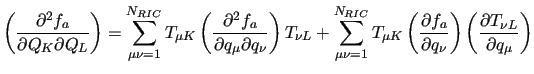$$\left( \frac{\partial^2f_a}{\partial Q_K\partial Q_L}\right) = \s... ...rtial q_{\nu}} \right) \left( \frac{\partial T_{\nu L}}{\partial q_\mu} \right)$$ (43)

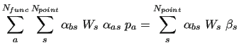
As shown in equation (6), the FF is linear in the $p$ parameters, thus the least squares minimization of functional (35) can be written as

$$\sum_a^{N_{func}} \sum_s^{N_{point}} \alpha_{bs} \ W_s \ \alpha_{as}\ p_a = \sum_s^{N_{point}} \alpha_{bs}\ W_s\ \beta_s$$ (44)

where the index $s$ runs over the collections $[g]$, $[Kg]$ and $[KLg]$ defined in equation (35) for energy, gradient and Hessian, respectively. Following this notation the matrix $\alpha$ and the vector $\beta$ are defined as

$$\alpha_{as} = f_{as} ~{\rm {or}}~ f_{as}^{\prime}~ {\rm {or}}~ f_... ...~ ; ~~~ \beta_s = E_s ~{\rm {or}}~ E_s^{\prime}~ {\rm {or}}~ E_s^{\prime\prime}$$

and

$$W_s = W_s ~{\rm {or}}~ \frac{W_s^{\prime}}{3N-6}~ {\rm {or}}~ \frac{W_s^{\prime\prime}}{(3N-6)(3N-5)}$$

where $f$'s are the functions of equation (6), $E$, $E^{\prime}$, $E^{\prime\prime}$ the QM data and $W$, $W^{\prime}$, $W^{\prime\prime}$ the weights of the merit function (35). Thus, defining

$$A = \alpha W \widetilde{\alpha}$$

$$b = \alpha W \beta$$

one has to solve a standard linear equation in the form

$$A p=b$$ (45)

where $A$ is a symmetric matrix.

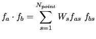
In usual FF it is convenient for practical purposes, to employ functions of the RIC that will be in general redundant over the considered points. The scalar product between the FF functions is defined as

$$f_a \cdot f_b = \sum_{s=1}^{N_{point}}W_s f_{as} \ f_{bs}$$ (46)

and the redundancy strongly depends on the number and type of points included in the fitting. However in general the $f$ set might not be linearly independent. This leads to a singular $A$ matrix and the direct inversion method can not be used to solve the linear system (45). On the contrary, the Singular Value Decomposition method [37,38] adapted to symmetric matrices is adequate and provides a stable solution of the linear system.