Force-field model potential functions
Once the set of RIC to be employed has been chosen, the analytical form of the model potential energy functions depending on the selected RIC must be declared.
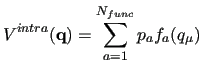
In the JOYCE code, the intramolecular FF is thus expressed as a sum of different terms, namely
 |
|
|
(6) |
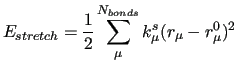
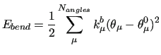
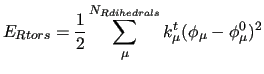
The first three terms count for the stiff IC, i.e. bond stretchings, angle bendings and stiff angle dihedrals (
 ), as those that drive the planarity of aromatic rings and are expressed with harmonic potentials:
 |
|
|
(7) |
 |
|
|
(8) |
 |
|
|
(9) |
Conversely, the model functions employed for soft, flexible dihedrals (
 ) are sums of periodic functions, namely
![$\displaystyle E_{Ftors} = \sum_\mu^{N_{Fdihedrals}}
\sum^{N_{cos_\mu}}_{j=1}
k^{d}_{j\mu}
\big[ 1 + \cos ( n_j^\mu \delta_\mu - \gamma_j^\mu ) \big]$](img133.png) |
|
|
(10) |
where
 is the number of cosine function employed to describe the potential of the
 dihedral.
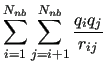
Finally, if any internal distance between atoms not directly bonded to each other is defined, the non-bonded intramolecular contribution is computed as
dihedral.
Finally, if any internal distance between atoms not directly bonded to each other is defined, the non-bonded intramolecular contribution is computed as
Note that, at difference with intermolecular energy terms
reported in equations (3) and (4),
 and
and  indexes run over atoms of the same molecule,
therefore
indexes run over atoms of the same molecule,
therefore  , to avoid self interaction. Furthermore,
the interaction parameters
, to avoid self interaction. Furthermore,
the interaction parameters
 and
and
 do not have to be necessarily the same
employed in the intermolecular LJ interaction reported in equation
(4), although some MD software do not allow to use different LJ parameters for intra and inter-molecular interactions.
do not have to be necessarily the same
employed in the intermolecular LJ interaction reported in equation
(4), although some MD software do not allow to use different LJ parameters for intra and inter-molecular interactions.
All of the aforementioned FF terms are expressed as sums of contribution, each depending on a single IC (even if, as before stated,  can always be expressed as a function of other generalized IC's).
If the last term of equation (6) is not included,
such FF is often termed as diagonal.
As a matter of fact the
can always be expressed as a function of other generalized IC's).
If the last term of equation (6) is not included,
such FF is often termed as diagonal.
As a matter of fact the  term, takes explicitly into account the coupling of two (or more) RIC.
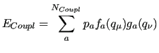
Since 2018, [21] the JOYCEcode has been equipped to handle two-variable functions designed to explicitly account for the coupling between the considered ICs.
As the detailed in the original paper, [21] a more convenient formalism can be adopted to clarify the coupling functions that can be used within the JOYCEparameterization procedure.
In fact, when the couling term is missing, the intramolecular energy of a purely diagonal
FF can be re-written as
term, takes explicitly into account the coupling of two (or more) RIC.
Since 2018, [21] the JOYCEcode has been equipped to handle two-variable functions designed to explicitly account for the coupling between the considered ICs.
As the detailed in the original paper, [21] a more convenient formalism can be adopted to clarify the coupling functions that can be used within the JOYCEparameterization procedure.
In fact, when the couling term is missing, the intramolecular energy of a purely diagonal
FF can be re-written as
 |
|
|
(12) |
where  stands for any internal coordinate
 reported in equations (7)-(10),
 refers to the force constant (either
  ,
,  , ...), while
  is the diagonal
potential function (
is the diagonal
potential function (
![$ [r_\mu - r_\mu^0]^2$](img150.png) ,
,
![$ [\theta_\mu - \theta_\mu^0]^2$](img151.png) ,
,
![$ [ 1 + \cos (n_j \delta_\mu - \gamma_j)]$](img152.png) , etc.) assigned to .
Within this framework, the generalized coupling introduced in JOYCEconsists in a sum of
, etc.) assigned to .
Within this framework, the generalized coupling introduced in JOYCEconsists in a sum of  pairwise linear terms, defined as the product
between two functions,
pairwise linear terms, defined as the product
between two functions,  and
and  , each depending only on one of the coupled ICs:
 |
|
|
(13) |
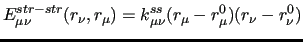
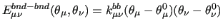
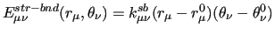
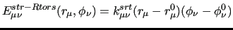
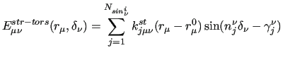
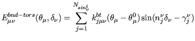
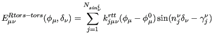
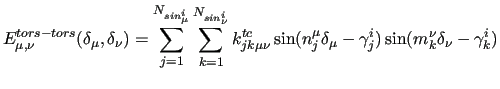
Following this notation, the coupling terms between two stiff ICs, are expressed by a product of linear terms involving each considered coordinate, as for instance:
 |
|
|
(14) |
 |
|
|
(15) |
 |
|
|
(16) |
 |
|
|
(17) |
While similar expressions can be easily derived for all couplings involving stiff ICs, for the sake of clarity, we describe in more detail the effect of coupling a stiff coordinate with a soft one, as
for instance a selected dihedral angle
 and a neighboring stretching distance,
  .
If we adopt a linear form for the term related to the stiff coordinate,
.
If we adopt a linear form for the term related to the stiff coordinate,
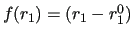 ,
and merge the coefficient and the function related to the soft coordinate into a generic function
,
and merge the coefficient and the function related to the soft coordinate into a generic function
 , equation (13) leads to
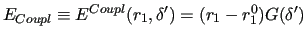 |
|
|
(18) |
The shape of
should be flexible enough so as to reproduce the reference profiles obtained by QM calculations.
In this sense, a Fourier series can again provide the required flexibility, together with other desirable features. [21]
All requisites can be verified using the functional form:
![$\displaystyle G(\delta^\prime) = \sum_i
k^{c}_i [1 + \sin(n_i \delta^\prime - \gamma^c_i)]$](img165.png) |
|
|
(19) |
which leads, to the following explicit coupling terms:
 |
|
|
(20) |
 |
|
|
(21) |
 |
|
|
(22) |
 |
|
|
(23) |
![$\displaystyle \sum^{N_{nb}}_{i=1} \sum^{N_{nb}}_{j=i+1}
4 \epsilon_{ij}^{intra}...
...} } \bigg )^{12} -
\bigg(\frac{ \sigma_{ij}^{intra} } {r_{ij} } \bigg)^6 \bigg]$](img137.png)